《Python深度学习》笔记整理:第二部分 深度学习实践——函数API与生成网络
代码基于 Keras 框架
函数API
函数API
函数API
Sequential 模型假设,网络只有一个输入和一个输出,而且网络是层的线性堆叠
网络结构为通常有向无环图
使用函数式 API 直接操作张量,或把层当作函数来使用,接收张量并返回张量
1
2
3
4
5
6
7
8
9
10
11
12
# Sequential模型
seq_model = Sequential()
seq_model.add(layers.Dense(32, activation='relu', input_shape=(64,)))
seq_model.add(layers.Dense(32, activation='relu'))
seq_model.add(layers.Dense(10, activation='softmax'))
# 函数API
input_tensor = Input(shape=(64,))
x = layers.Dense(32, activation='relu')(input_tensor)
x = layers.Dense(32, activation='relu')(x)
output_tensor = layers.Dense(10, activation='softmax')(x)
model = Model(input_tensor, output_tensor) # 将输入张量和输出张量转换为一个模型如果试图利用不相关的输入和输出来构建一个模型,会报错 RuntimeError
进行编译、训练或评估时,其 API 与 Sequential 模型相同
多输入
在某一时刻用一个可以组合多个张量的层将不同的输入分支合并,如相加、连接
双输入的问答模型
1
2
3
4
5
6
7
8
9
10
11
12
13
14
15
16
17
18
19
20
21
22
23
24
25
26
27
28
29
30
31
32
33
34
35
36
from keras.models import Model
from keras import layers
from keras import Input
text_vocabulary_size = 10000
question_vocabulary_size = 10000
answer_vocabulary_size = 500
# 参考文本的输入
text_input = Input(shape=(None,), dtype='int32', name='text') # 文本输入,可对输入命名
embedded_text = layers.Embedding(
text_vocabulary_size, 64)(text_input)
encoded_text = layers.LSTM(32)(embedded_text)
# 问题的输入
question_input = Input(shape=(None,),
dtype='int32',
name='question') # 使用不同的层实例
embedded_question = layers.Embedding(question_vocabulary_size,
32)(question_input)
encoded_question = layers.LSTM(16)(embedded_question)
# 编码后的问题和文本连接起来
concatenated = layers.concatenate([encoded_text, encoded_question],
axis=-1)
answer = layers.Dense(answer_vocabulary_size,
activation='softmax')(concatenated)
model = Model([text_input, question_input], answer) # 指定两个输入和输出
model.compile(optimizer='rmsprop',
loss='categorical_crossentropy',
metrics=['acc'])
...
# 模型输入
model.fit([text, question], answers, epochs=10, batch_size=128) # 输入组成的列表
model.fit({'text': text, 'question': question}, answers,
epochs=10, batch_size=128) # 输入组成的字典,必须对输入进行命名
多输出
一个网络试图同时预测数据的不同性质
三输出模型
1
2
3
4
5
6
7
8
9
10
11
12
13
14
15
16
17
18
19
20
21
22
23
24
25
26
27
from keras import layers
from keras import Input
from keras.models import Model
vocabulary_size = 50000
num_income_groups = 10
posts_input = Input(shape=(None,), dtype='int32', name='posts')
embedded_posts = layers.Embedding(256, vocabulary_size)(posts_input)
x = layers.Conv1D(128, 5, activation='relu')(embedded_posts)
x = layers.MaxPooling1D(5)(x)
x = layers.Conv1D(256, 5, activation='relu')(x)
x = layers.Conv1D(256, 5, activation='relu')(x)
x = layers.MaxPooling1D(5)(x)
x = layers.Conv1D(256, 5, activation='relu')(x)
x = layers.Conv1D(256, 5, activation='relu')(x)
x = layers.GlobalMaxPooling1D()(x)
x = layers.Dense(128, activation='relu')(x)
# 输出层都具有名称
age_prediction = layers.Dense(1, name='age')(x)
income_prediction = layers.Dense(num_income_groups,
activation='softmax',
name='income')(x)
gender_prediction = layers.Dense(1, activation='sigmoid', name='gender')(x)
model = Model(posts_input,
[age_prediction, income_prediction, gender_prediction])损失函数要不同——使用损失组成的列表或字典来为不同输出指定不同损失,并指定损失的权重
1
2
3
4
5
6
7
8
9
10
11
12
13
14
15
16
17
# 列表
model.compile(optimizer='rmsprop',
loss=['mse', 'categorical_crossentropy', 'binary_crossentropy'],
loss_weights=[0.25, 1., 10.])
# 字典 要求输出层具有名字
model.compile(optimizer='rmsprop',
loss={'age': 'mse',
'income': 'categorical_crossentropy',
'gender': 'binary_crossentropy'},
loss_weights={'age': 0.25,
'income': 1.,
'gender': 10.})
# fit
model.fit(posts, {'age': age_targets,
'income': income_targets,
'gender': gender_targets},
epochs=10, batch_size=64)
有向无环图
Inception 模块:完整的Inception V3架构内置于 Keras,
keras.applications.inception_v3.InceptionV3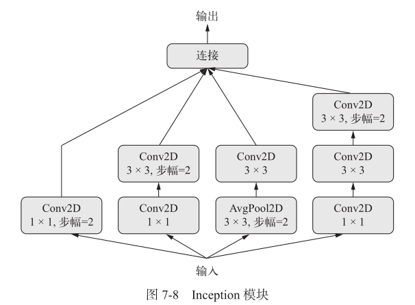
1
2
3
4
5
6
7
8
9
10
11
12
13
14
15
from keras import layers
# 每个分支都有相同的步幅值
branch_a = layers.Conv2D(128, 1,
activation='relu', strides=2)(x)
branch_b = layers.Conv2D(128, 1, activation='relu')(x)
branch_b = layers.Conv2D(128, 3, activation='relu', strides=2)(branch_b)
branch_c = layers.AveragePooling2D(3, strides=2)(x)
branch_c = layers.Conv2D(128, 3, activation='relu')(branch_c)
branch_d = layers.Conv2D(128, 1, activation='relu')(x)
branch_d = layers.Conv2D(128, 3, activation='relu')(branch_d)
branch_d = layers.Conv2D(128, 3, activation='relu', strides=2)(branch_d)
# 分支输出连接在一起
output = layers.concatenate(
[branch_a, branch_b, branch_c, branch_d], axis=-1)残差连接
解决梯度消失和表示瓶颈
让前面某层的输出作为后面某层的输入
前面层的输出没有与后面层的激活连接,而是与后面层的激活相加——前提是激活的形状相同,否则用线性变换将前面层的输出改为目标形状
尺寸相同
1
2
3
4
5
6
7
8
from keras import layers
x = ...
y = layers.Conv2D(128, 3, activation='relu', padding='same')(x)
y = layers.Conv2D(128, 3, activation='relu', padding='same')(y)
y = layers.Conv2D(128, 3, activation='relu', padding='same')(y)
y = layers.add([y, x]) # 原始x与输出特征相加尺寸不同
1
2
3
4
5
6
7
8
9
10
from keras import layers
x = ...
y = layers.Conv2D(128, 3, activation='relu', padding='same')(x)
y = layers.Conv2D(128, 3, activation='relu', padding='same')(y)
y = layers.MaxPooling2D(2, strides=2)(y)
residual = layers.Conv2D(128, 1, strides=2, padding='same')(x)
y = layers.add([y, residual]) # 将原始x张量线性下采样,使其与y具有相同的形状
共享层权重
几个分支全都共享相同的知识并执行相同的运算,并同时对不同的输入集合学习这些表示
评估两个句子的语义相似度:两个句子可以互换,因为相似度是对称的关系
1
2
3
4
5
6
7
8
9
10
11
12
13
14
15
16
17
from keras import layers
from keras import Input
from keras.models import Model
lstm = layers.LSTM(32) # 实例化一个LSTM层
# 构建模型的左分支
left_input = Input(shape=(None, 128))
left_output = lstm(left_input)
# 构建模型的右分支
right_input = Input(shape=(None, 128))
right_output = lstm(right_input) # 调用已有的层实例,重复使用它的权重
# 构建一个分类器
merged = layers.concatenate([left_output, right_output], axis=-1)
predictions = layers.Dense(1, activation='sigmoid')(merged)
model = Model([left_input, right_input], predictions)
model.fit([left_data, right_data], targets)
模型视为层
在一个输入张量上调用模型,并得到一个输出张量;或者模型具有多个输入张量和多个输出张量,此时用张量列表调用模型
共享卷积基
1
2
3
4
5
6
7
8
9
10
11
12
13
14
15
from keras import layers
from keras import applications
from keras import Input
# 实例化Xception网络(只有卷积基)
xception_base = applications.Xception(weights=None,
include_top=False)
left_input = Input(shape=(250, 250, 3))
right_input = Input(shape=(250, 250, 3))
# 相同的视觉模型调用两次
left_features = xception_base(left_input)
right_features = xception_base(right_input)
merged_features = layers.concatenate(
[left_features, right_features], axis=-1)
TensorBoard
回调函数
keras.callback模块在调用
fit时传入模型的一个对象(实现特定方法的类实例) ,在训练过程中的不同时间点被模型调用,访问模型状态与性能数据, 并采取一些行动- 模型检查点(model checkpointing) :在训练过程中的不同时间点保存模型的当前权重
- 提前终止(early stopping) :如果验证损失不再改善,则中断训练,并保存模型
- 训练过程中动态调节某些参数值:如优化器的学习率
- 训练过程中记录训练指标和验证指标,或将模型学到的表示可视化
ModelCheckpoint 与 EarlyStopping
1
2
3
4
5
6
7
8
9
10
11
12
13
14
15
16
17
18
19
20
21
22
23
24
import keras
callbacks_list = [
keras.callbacks.EarlyStopping(
monitor='acc', # 监控模型的验证精度
patience=1, # 精度在多于一轮的时间(即两轮)内不再改善则停止训练
),
keras.callbacks.ModelCheckpoint( # 每轮过后保存当前权重
filepath='my_model.h5', # 目标模型文件的保存路径
# val_loss没有改善,则不覆盖模型文件
monitor='val_loss',
save_best_only=True,
)
]
model.compile(optimizer='rmsprop',
loss='binary_crossentropy',
metrics=['acc'])
# 回调函数要监控验证损失和验证精度,因此必须传入验证数据
model.fit(x, y,
epochs=10,
batch_size=32,
callbacks=callbacks_list,
validation_data=(x_val, y_val))ReduceLROnPlateau:验证损失不再改善时,说明陷入损失平台,使用这个回调函数来降低(增大)学习率,跳出局部最小值
1
2
3
4
5
6
7
callbacks_list = [
keras.callbacks.ReduceLROnPlateau(
monitor='val_loss' # 监控模型验证损失
factor=0.1, # 触发时将学习率除以 10
patience=10, # 验证损失在10轮内没有改善时触发此回调函数
)
]编写自己的回调函数
创建
keras.callbacks.Callback类的子类on_epoch_begin:每轮开始时被调用on_epoch_end:每轮结束时被调用on_batch_begin:处理每个批量之前被调用on_batch_end:处理每个批量之后被调用on_train_begin:训练开始时被调用on_train_end:训练结束时被调用
示例:每轮结束时保存对验证集第一个样本每层的激活,格式为 Numpy
1
2
3
4
5
6
7
8
9
10
11
12
13
14
15
16
17
18
19
import keras
import numpy as np
class ActivationLogger(keras.callbacks.Callback):
def set_model(self, model):
self.model = model # 训练之前由父模型调用,告诉回调函数哪个模型在调用
layer_outputs = [layer.output for layer in model.layers]
self.activations_model = keras.models.Model(model.input,
layer_outputs) # 模型实例,返回每层的激活
# log参数是一个字典,里面包含前一个批量、前一个轮次或前一次训练的信息, 即训练指标和验证指标等
def on_epoch_end(self, epoch, logs=None):
if self.validation_data is None:
raise RuntimeError('Requires validation_data.')
validation_sample = self.validation_data[0][0:1] # 获取验证数据的第一个样本
activations = self.activations_model.predict(validation_sample)
f = open('activations_at_epoch_' + str(epoch) + '.npz', 'w')
np.savez(f, activations)
f.close()
TensorBoard
需要创建一个目录,保存它生成的日志文件
用 TensorBoard 回调函数实例启动训练
1
2
3
4
5
6
7
8
9
10
11
12
callbacks = [
keras.callbacks.TensorBoard(
log_dir='my_log_dir', # 日志文件写入位置
histogram_freq=1, # 每一轮之后记录激活直方图
embeddings_freq=1, # 每一轮后记录嵌入数据
)
]
history = model.fit(x_train, y_train,
epochs=20,
batch_size=128,
validation_split=0.2,
callbacks=callbacks)启动
1
$ tensorboard --logdir=my_log_dir
将模型绘制为层组成的图
1
2
3
4
5
from keras.utils import plot_model
plot_model(model, to_file='model.png')
# 显示每一层的形状信息
plot_model(model, show_shapes=True, to_file='model.png')
模型性能提高
高级架构模式
批标准化
有助于梯度传播
通常在卷积层或密集连接层之后使用
接收
axis参数,默认为-1,即张量最后一个轴1
2
3
4
5conv_model.add(layers.Conv2D(32, 3, activation='relu'))
conv_model.add(layers.BatchNormalization())
dense_model.add(layers.Dense(32, activation='relu'))
dense_model.add(layers.BatchNormalization())
深度可分离卷积:比 CNN 更快,但假设输入中的空间位置高度相关、不同的通道之间相对独立
1
2
3
4
5
6
7
8
9
10
11
12
13
14
15
16
17
18
19
20
21
22
23
24
25
26
27from keras.models import Sequential, Model
from keras import layers
height = 64
width = 64
channels = 3
num_classes = 10
model = Sequential()
model.add(layers.SeparableConv2D(32, 3,
activation='relu',
input_shape=(height, width, channels,)))
model.add(layers.SeparableConv2D(64, 3, activation='relu'))
model.add(layers.MaxPooling2D(2))
model.add(layers.SeparableConv2D(64, 3, activation='relu'))
model.add(layers.SeparableConv2D(128, 3, activation='relu'))
model.add(layers.MaxPooling2D(2))
model.add(layers.SeparableConv2D(64, 3, activation='relu'))
model.add(layers.SeparableConv2D(128, 3, activation='relu'))
model.add(layers.GlobalAveragePooling2D())
model.add(layers.Dense(32, activation='relu'))
model.add(layers.Dense(num_classes, activation='softmax'))
model.compile(optimizer='rmsprop', loss='categorical_crossentropy')
超参数优化
- 过程如下
- 选择一组超参数
- 构建相应的模型
- 训练并衡量验证数据性能
- 自动选择下一组超参数
- 重复
- 衡量测试集上性能
模型集成
- 多个子模型共同决定一个结果
- 平均或加权决定最终结果
生成网络
LSTM 生成文本
使用前面的标记作为输入,训练一个网络(通常是循环神经网络或卷积神经网络)来预测序列中接下来的一个或多个标记
采样策略
- 贪婪采样:始终选择可能性最大的下一个字符
- 随机采样:从下一个字符的概率分布中进行采样
引入 softmax 温度(softmax temperature)控制采样时随机性的大小,即表示所选择的下一个字符会有多么出人意料(越大,则越出人意料)
1
2
3
4
5
6import numpy as np
# 第一个参数为softmax的分布结果
def reweight_distribution(original_distribution, temperature=0.5):
distribution = np.log(original_distribution) / temperature
distribution = np.exp(distribution)
return distribution / np.sum(distribution) # 返回原始分布重新加权后的结果,除以求和是为了让其和保持1字符级文本生成(一维卷积也可生成字符)
解析初始文本文件
字符序列向量化(独热编码)
构建网络
1
2
3
4
5
6
7from keras import layers
model = keras.models.Sequential()
model.add(layers.LSTM(128, input_shape=(maxlen, len(chars))))
model.add(layers.Dense(len(chars), activation='softmax'))
optimizer = keras.optimizers.RMSprop(lr=0.01)
model.compile(loss='categorical_crossentropy', optimizer=optimizer)训练并采样
根据文本,生成下一个字符概率分布
分布重新加权
随机采样
添加到文本尾部
1
2
3
4
5
6
7
8
9
10
11
12
13
14
15
16
17
18
19
20
21
22
23
24
25
26
27
28
29
30
31
32
33
34
35
36
37# 采样下一个字符
def sample(preds, temperature=1.0):
preds = np.asarray(preds).astype('float64')
preds = np.log(preds) / temperature
exp_preds = np.exp(preds)
preds = exp_preds / np.sum(exp_preds)
probas = np.random.multinomial(1, preds, 1)
return np.argmax(probas)
# 文本生成循环,一边训练,一边生成文本
import random
import sys
for epoch in range(1, 60):
print('epoch', epoch)
model.fit(x, y, batch_size=128, epochs=1) # 拟合一次
# 随机选择一个文本种子
start_index = random.randint(0, len(text) - maxlen - 1)
generated_text = text[start_index: start_index + maxlen]
print('--- Generating with seed: "' + generated_text + '"')
for temperature in [0.2, 0.5, 1.0, 1.2]: # 尝试一系列不同采样温度
print('------ temperature:', temperature)
sys.stdout.write(generated_text)
for i in range(400): # 从种子文本开始,生成400个字符
# 生成的字符 one-hot 编码
sampled = np.zeros((1, maxlen, len(chars)))
for t, char in enumerate(generated_text):
sampled[0, t, char_indices[char]] = 1.
# 对下一个字符采样
preds = model.predict(sampled, verbose=0)[0]
next_index = sample(preds, temperature)
next_char = chars[next_index]
generated_text += next_char
generated_text = generated_text[1:]
sys.stdout.write(next_char)
迁移
- 风格(style)指图像中不同空间尺度的纹理、颜色和视觉图案,内容(content)指图像的高级宏观结构
- 网络更靠底部的层激活包含关于图像的局部信息,而更靠近顶部的层则包含更加全局、更加抽象的信息
- 内容损失:预训练的卷积神经网络更靠顶部的某层在目标图像上计算得到的激活,同一层在生成图像上计算得到的激活,二者的 L2 范数
- 风格损失:
- 目标内容图像和生成图像之间保持相似的较高层激活
- 较低层和较高层的激活中保持类似的相互关系
风格迁移实现(VGG19 网络为例)
创建一个网络,同时计算风格参考图像、目标图像和生成图像的 VGG19 层激活
网络接收三张图像的批量,分别是风格参考图像、目标图像和一个用于保存生成图像的占位符
1
2
3
4
5
6
7
8
9
10
11
12
13
14from keras import backend as K
target_image = K.constant(preprocess_image(target_image_path))
style_reference_image = K.constant(preprocess_image(style_reference_image_path))
combination_image = K.placeholder((1, img_height, img_width, 3))
input_tensor = K.concatenate([target_image,
style_reference_image,
combination_image], axis=0)
model = vgg19.VGG19(input_tensor=input_tensor,
weights='imagenet',
include_top=False)
print('Model loaded.')定义内容损失:目标图像和生成图像在 VGG19 卷积神经网络的顶层具有相似的结果
1
2def content_loss(base, combination):
return K.sum(K.square(combination - base))定义风格损失:
1
2
3
4
5
6
7
8
9
10
11
12# 计算输入矩阵的格拉姆矩阵——原始特征矩阵中相互关系的映射
def gram_matrix(x):
features = K.batch_flatten(K.permute_dimensions(x, (2, 0, 1)))
gram = K.dot(features, K.transpose(features))
return gram
def style_loss(style, combination):
S = gram_matrix(style)
C = gram_matrix(combination)
channels = 3
size = img_height * img_width
return K.sum(K.square(S - C)) / (4. * (channels ** 2) * (size ** 2))定义总变差损失:使生成图像具有空间连续性,可以理解为正则化损失
1
2
3
4
5
6
7
8def total_variation_loss(x):
a = K.square(
x[:, :img_height - 1, :img_width - 1, :] -
x[:, 1:, :img_width - 1, :])
b = K.square(
x[:, :img_height - 1, :img_width - 1, :] -
x[:, :img_height - 1, 1:, :])
return K.sum(K.pow(a + b, 1.25))定义最终的损失
1
2
3
4
5
6
7
8
9
10
11
12
13
14
15
16
17
18
19
20
21
22
23
24
25
26
27
28
29
30# 层的名称映射为激活张量的字典
outputs_dict = dict([(layer.name, layer.output) for layer in model.layers])
# 用于内容损失的层
content_layer = 'block5_conv2'
# 用于风格损失的层
style_layers = ['block1_conv1',
'block2_conv1',
'block3_conv1',
'block4_conv1',
'block5_conv1']
# 损失分量的加权平均所使用的权重
total_variation_weight = 1e-4
style_weight = 1.
content_weight = 0.025
# 内容损失
loss = K.variable(0.)
layer_features = outputs_dict[content_layer]
target_image_features = layer_features[0, :, :, :]
combination_features = layer_features[2, :, :, :]
loss += content_weight * content_loss(target_image_features,
combination_features)
# 添加每个目标层的风格损失分量
for layer_name in style_layers:
layer_features = outputs_dict[layer_name]
style_reference_features = layer_features[1, :, :, :]
combination_features = layer_features[2, :, :, :]
sl = style_loss(style_reference_features, combination_features)
loss += (style_weight / len(style_layers)) * sl
# 添加总变差损失
loss += total_variation_weight * total_variation_loss(combination_image)设置梯度下降
1
2
3
4
5
6
7
8
9
10
11
12
13
14
15
16
17
18
19
20
21
22
23
24
25
26
27# 获取损失相对于生成图像的梯度
grads = K.gradients(loss, combination_image)[0]
# 获取当前损失值和当前梯度值的函数
fetch_loss_and_grads = K.function([combination_image], [loss, grads])
class Evaluator(object):
def __init__(self):
self.loss_value = None
self.grads_values = None
def loss(self, x):
assert self.loss_value is None
x = x.reshape((1, img_height, img_width, 3))
outs = fetch_loss_and_grads([x])
loss_value = outs[0]
grad_values = outs[1].flatten().astype('float64')
self.loss_value = loss_value
self.grad_values = grad_values
return self.loss_value
def grads(self, x):
assert self.loss_value is not None
grad_values = np.copy(self.grad_values)
self.loss_value = None
self.grad_values = None
return grad_values
evaluator = Evaluator()风格迁移循环
1
2
3
4
5
6
7
8
9
10
11
12
13
14
15
16
17
18
19from scipy.optimize import fmin_l_bfgs_b
from scipy.misc import imsave
import time
result_prefix = 'my_result'
iterations = 20
x = preprocess_image(target_image_path) # 目标图像
x = x.flatten() # 图像展平,scipy.optimize.fmin_l_bfgs_b 只能处理展平的向量
for i in range(iterations):
print('Start of iteration', i)
start_time = time.time()
# L-BFGS 最优化,以将神经风格损失最小化;计算损失的函数和计算梯度的函数作为单独的参数传入
x, min_val, info = fmin_l_bfgs_b(evaluator.loss,
x,
fprime=evaluator.grads,
maxfun=20)
# 保存图片
...
变分自编码器
从潜在空间采样
- VAE 非常适合用于学习具有良好结构的潜在空间,其中特定方向表示数据中有意义的变化轴
- 自编码器是一种网络类型,其目的是将输入编码到低维潜在空间,然后再解码回来
- 经典的图像自编码器接收一张图像,通过一个编码器模块将其映射到潜在向量空间,然后再通过一个解码器模块将其解码为与原始图像具有相同尺寸的输出。使用与输入图像相同的图像作为目标数据来训练这个自编码器——学习对原始输入进行重新构建
VAE
VAE 向自编码器添加了一点统计限制,迫使其学习连续的、高度结构化的潜在空间——将图像转换为统计分布的参数
假设输入图像是由统计过程生成的,VAE 使用平均值和方差两个参数从分布中随机采样一个元素,并将这个元素解码到原始输入。这迫使潜在空间的任何位置都对应有意义的表示,即潜在空间采样的每个点都能解码为有
效的输出通过两个损失函数进行训练:
重构损失(reconstruction loss):迫使解码后的样本匹配初始输入
正则化损失(regularization loss):有助于学习具有良好结构的潜在空间,并降低训练数据上的过拟合
1
2
3
4
5
6
7z_mean, z_log_variance = encoder(input_img)
# 使用小随机数epsilon来抽取一个潜在点
z = z_mean + exp(z_log_variance) * epsilon
reconstructed_img = decoder(z)
model = Model(input_img, reconstructed_img)
编码器
1
2
3
4
5
6
7
8
9
10
11
12
13
14
15
16
17
18
19
20
21
22
23
24
25
26
27
28import keras
from keras import layers
from keras import backend as K
from keras.models import Model
import numpy as np
img_shape = (28, 28, 1)
batch_size = 16
latent_dim = 2 # 假设潜在空间为一个二维平面
input_img = keras.Input(shape=img_shape)
x = layers.Conv2D(32, 3,
padding='same', activation='relu')(input_img)
x = layers.Conv2D(64, 3,
padding='same', activation='relu',
strides=(2, 2))(x)
x = layers.Conv2D(64, 3,
padding='same', activation='relu')(x)
x = layers.Conv2D(64, 3,
padding='same', activation='relu')(x)
shape_before_flattening = K.int_shape(x)
x = layers.Flatten()(x)
x = layers.Dense(32, activation='relu')(x)
# 输入图像被编码为两个参数
z_mean = layers.Dense(latent_dim)(x)
z_log_var = layers.Dense(latent_dim)(x)潜在空间采样——任何对象都应该是一个层, 如果代码不是内置层的一部分, 应该将其包装到一个 Lambda 层
1
2
3
4
5
6
7def sampling(args):
z_mean, z_log_var = args
epsilon = K.random_normal(shape=(K.shape(z_mean)[0], latent_dim),
mean=0., stddev=1.)
return z_mean + K.exp(z_log_var) * epsilon
z = layers.Lambda(sampling)([z_mean, z_log_var])解码器
1
2
3
4
5
6
7
8
9
10
11
12
13
14
15
16
17
18decoder_input = layers.Input(K.int_shape(z)[1:])
x = layers.Dense(np.prod(shape_before_flattening[1:]),
activation='relu')(decoder_input) # 对输入进行上采样
x = layers.Reshape(shape_before_flattening[1:])(x)
# 将z 解码为与原始输入图像具有相同尺寸的特征图
x = layers.Conv2DTranspose(32, 3,
padding='same',
activation='relu',
strides=(2, 2))(x)
x = layers.Conv2D(1, 3,
padding='same',
activation='sigmoid')(x)
# 解码器模型实例化
decoder = Model(decoder_input, x)
z_decoded = decoder(z)计算损失的自定义层
1
2
3
4
5
6
7
8
9
10
11
12
13
14
15
16
17
18class CustomVariationalLayer(keras.layers.Layer):
def vae_loss(self, x, z_decoded):
x = K.flatten(x)
z_decoded = K.flatten(z_decoded)
xent_loss = keras.metrics.binary_crossentropy(x, z_decoded)
kl_loss = -5e-4 * K.mean(
1 + z_log_var - K.square(z_mean) - K.exp(z_log_var), axis=-1)
return K.mean(xent_loss + kl_loss)
def call(self, inputs):
x = inputs[0]
z_decoded = inputs[1]
loss = self.vae_loss(x, z_decoded)
self.add_loss(loss, inputs=inputs)
return x # 不使用这个值,但层必须要有返回值
y = CustomVariationalLayer()([input_img, z_decoded])
GAN
- 替代 VAE 学习图像的潜在空间,但这个潜在空间无法保证具有有意义的结构,而且是不连续的
- 分为生成器网络和判别器网络
- 最优化过程寻找的不是一个最小值,而是一个平衡
- gan 网络将 generator 网络和 discriminator 网络连接在一起:gan(x) = discriminator(generator(x))。生成器将潜在空间向量解码为图像,判别器对这些图像的真实性进行评估
相关技巧
tanh 作为生成器最后一层的激活, 而不用 sigmoid
使用正态分布(高斯分布)对潜在空间中的点进行采样
在训练过程中引入随机性
- 向判别器的标签添加随机噪声
- 在判别器中使用 dropout
稀疏的梯度会妨碍训练
- 使用步进卷积代替最大池化来进行下采样
- 使用 LeakyReLU 层来代替 ReLU 激活
每当在生成器和判别器中都使用步进的卷积时,内核大小要被步幅大小整除
生成器
1 | import keras |
判别器
1 | discriminator_input = layers.Input(shape=(height, width, channels)) |
对抗网络
模型将潜在空间的点转换为一个分类决策,训练的标签都是“真实图像”
训练过程中需要将判别器设置为冻结
1 | discriminator.trainable = False |
训练
- 对抗损失开始大幅增加,而判别损失则趋向于零——判别器最终支配了生成器——尝试减小判别器的学习率, 并增大判别器的 dropout 比率
1 | import os |